3 Results
Four findings emerge from the canonical configuration (seed 17, \(dt = 3.0\)) and build in sequence. First, that pollution is structurally delayed behind the capital boom (Section 3.1) — this is the mechanism that drives everything else. Second, that all three P-triggered levers fail precisely because that delay is irreducible (Section 3.2). Third, that the same cap instrument succeeds when triggered on capital instead, producing a Pareto-improving win-win (Section 3.3). Fourth, that triggering earlier monotonically increases the benefit to both emitter and downwind arenas (Section 3.4). A fifth subsection (Section 3.5) collects the shared mechanism across all four. Chapter 4 then tests generality across parameter perturbations. Throughout, downwind recovery denotes arena B’s relative peak-capital gain over the no-governance control, \(\mathrm{recover}_B = 100\,(B^{\mathrm{peak}}_{\mathrm{gov}} - B^{\mathrm{peak}}_{\mathrm{ctrl}}) / B^{\mathrm{peak}}_{\mathrm{ctrl}}\), so \(0\,\%\) means no improvement and a later, higher B peak raises it.
3.1 Pollution is the lagging tail of the boom
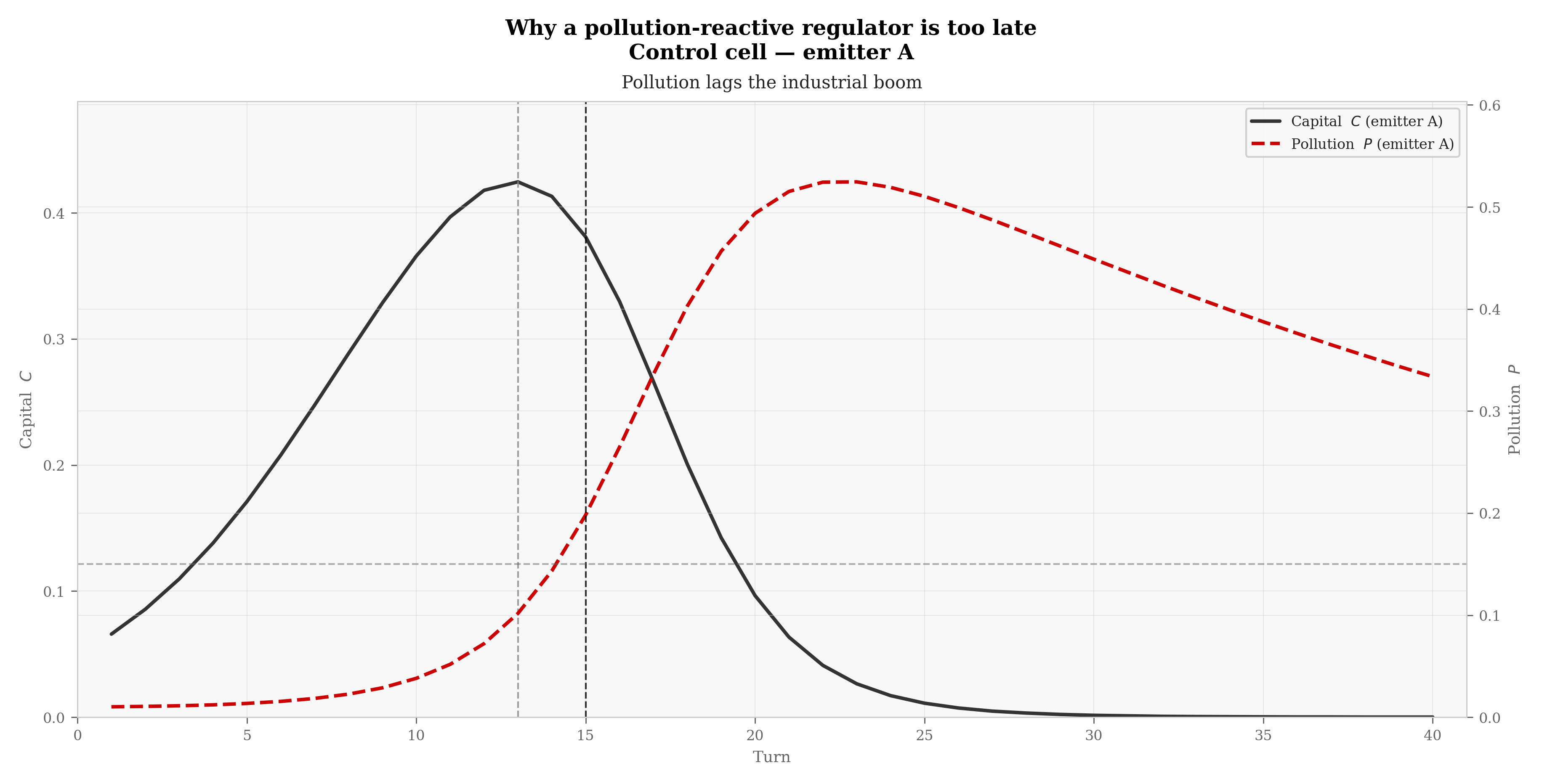
The control cell (Figure 3.1) — three arenas coupled by pollution links, no governance — reproduces the Seneca cascade. Emitter A’s capital C peaks at 0.425 at t13; its pollution P crosses the 0.15 reactive threshold only at t15 (crossing the 0.05 mark at t11, when capital is already at 93 % of its peak), and continues rising to 0.525 at t23. The downwind arenas B and C are choked: their peak capital reaches only 0.114 (vs A’s 0.425), they collapse at t20, and their imported pollution peaks at 3.227 — roughly 7.1\(\times\) the pollution this downwind arena reaches in the un-cascaded control.
The 2-turn gap between capital peak (t13) and pollution reaching the reactive threshold (t15) is not a calibration accident — it follows from the ODE structure. Since \(dP/dt = k_2 C P\) (Eq. 2.1) is multiplicative in C, pollution can only accelerate after capital has already grown large. By the time P clears any non-trivial detection threshold, the industrial boom that will emit the rest of the pollutant is already committed. A regulator keyed on P is therefore structurally late, reacting to a symptom whose cause is already behind it.
3.2 Reactive (P-triggered) levers fail
When the regulator arms on pollution (P > 0.15) and applies a cap on the capital growth rate (\(k_1 \to 0.02\)), the outcome is nearly indistinguishable from the control (Table 3.1). A’s peak P drops marginally (0.525 \(\to\) 0.478, -9 %), B’s imported pollution peak falls from 3.227 to 2.967, and B’s peak capital improves by 0 %: the downwind arenas still die at t20. The cap arrives too late to dissolve the capital stock already built — regenset throttles future growth but cannot undo existing C, which continues to emit.
A stronger instrument on the same lagging trigger does not resolve the timing problem. When the regulator applies a levy (capital_shock, \(C \times 0.5\)) on the P-trigger, it claws back built capital more aggressively: A’s peak P halves (0.525 \(\to\) 0.236, -55 %), B’s imported pollution peak drops from 3.227 to 1.470 (-54 %). Yet B’s peak capital still shows 0 % improvement over the control — the levy arrives late and the halved dose is still too large for B’s smaller economy. Worse, stripping A’s capital pushes A’s collapse earlier (t17 vs t22 in the control), a perverse outcome in which reactive governance accelerates the emitter’s own demise without rescuing the victims.
The fine (wealth_shock on A’s households, wealth \(\times\) 0.5) serves as a negative control: it zeroes A’s households’ wealth by t22 but leaves P and B completely unchanged (peak P 0.525, B peak 0.114, B recovery 0 %). The failure is structural — Bardi’s ODE has no demand-to-production channel, so a consumption-side instrument cannot affect the autonomous capital C that generates pollution. This is a model limitation, not a policy claim (Chapter 5).
| Cell | A peak C | A peak P | A collapse | B peak C | B peak P (import) | B collapse | B recovery |
|---|---|---|---|---|---|---|---|
| control | 0.425 | 0.525 | t22 | 0.114 | 3.227 | t20 | — |
| cap-reactive | 0.425 | 0.478 | t22 | 0.114 | 2.967 | t20 | 0 % |
| levy-reactive | 0.425 | 0.236 | t17 | 0.114 | 1.470 | t21 | 0 % |
| fine (neg. ctrl) | 0.425 | 0.525 | t22 | 0.114 | 3.227 | t20 | 0 % |
3.2.1 P-threshold sweep: every reactive threshold is structurally too late
The cap-reactive cell tests one pollution threshold (P > 0.15), but the structural argument — \(dP/dt = k_2 \cdot C \cdot P\) is multiplicative in C, so P cannot rise until C is already large — implies that every governance-relevant \(P > \varepsilon\) should fire only once the capital boom is already well advanced. We confirm this with a sweep (Table 3.2) over five thresholds, P > 0.02 to P > 0.15, all otherwise identical to cap-reactive. The lowest meaningful threshold is P > 0.02: the emitter starts at \(P_0 = 0.01\), so nothing below that can ever fire. Yet even P > 0.02 does not cross until t8, when A’s capital already sits at 68 % of its eventual peak (0.289 of 0.425); P > 0.05 fires at t11 (93 %) and P > 0.10 exactly at the peak (t13, C = 0.425). Reacting earlier on the lagging signal helps only marginally: B’s recovery rises monotonically as the threshold falls but tops out at a trivial +1.4 % at P > 0.02 — B still collapses — and the emitter is never saved at any reactive threshold. The cascade is committed before pollution clears even its own starting level.
P > 0.02; the emitter’s pollution starts at \(P_0 = 0.01\)) fires only at t8, with capital already at 68 % of its peak, and still neither rescues the emitter nor lifts downwind recovery above a trivial +1.4 %.
| P threshold | Fires at | C at fire (% of C peak) | A collapse | B recovery |
|---|---|---|---|---|
| P > 0.02 | t8 | 0.289 (68 %) | t28 | +1.4 % |
| P > 0.03 | t10 | 0.366 (86 %) | t24 | +0.2 % |
| P > 0.05 | t11 | 0.397 (93 %) | t23 | 0 % |
| P > 0.10 | t13 | 0.425 (100 %, at peak) | t22 | 0 % |
| P > 0.15 | t15 | 0.381 (90 %, post-peak) | t22 | 0 % |
3.3 Leading (capital-triggered) regulation is the win
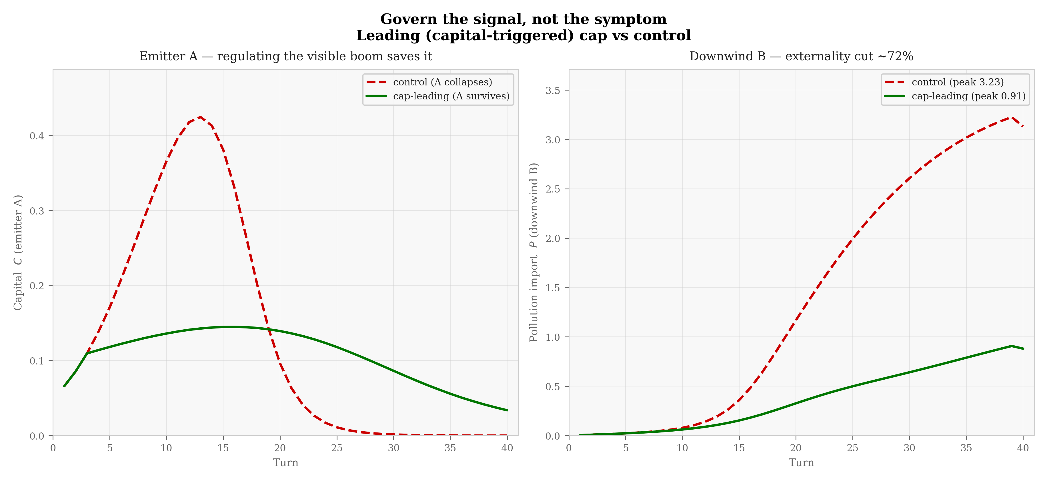
Arming the same \(k_1\) cap on the leading signal — C > 0.10, which fires at t3 — transforms the outcome (Figure 3.2). A survives: its capital never collapses (plateau at \(\approx\) 0.10–0.15), its peak P drops from 0.525 to 0.138 (-74 %). B’s imported pollution peak falls from 3.227 to 0.908 (-72 %), B’s peak capital improves to 0.136 (+19.7 % over the control), and B’s collapse is postponed from t20 to t27 (Table 3.3).
The mechanism is not that the cap is a better instrument than the levy — it is the same regenset as in Section 3.2. The difference is entirely in the trigger signal. By acting on capital at t3 (when C = 0.10 and \(P \approx 0.01\)), the regulator throttles growth before the pollution engine engages. The industrial boom never materialises, so the Seneca cliff never arrives — for the emitter or for its downwind neighbours. This is a Pareto improvement (hereafter win-win): regulating the emitter saves the emitter from its own Seneca cliff, not just the victims from the externality. Welfare is read here as integrated capital plus survival (consistent with a long-horizon undiscounted commons); under strong intertemporal discounting the boom-and-bust trajectory could be preferred to the plateau, but the cascade-and-collapse comparison itself is robust to that choice.
| Metric | Control | Cap-leading | \(\Delta\) |
|---|---|---|---|
| A peak C | 0.425 | 0.145 | -66 % |
| A peak P | 0.525 | 0.138 | -74 % |
| A survives | no (t22) | yes | — |
| B peak C | 0.114 | 0.136 | +19.7 % |
| B peak P (import) | 3.227 | 0.908 | -72 % |
| B collapse | t20 | t27 | +7 turns |
3.3.1 The 2x2 design: trigger column dominates instrument row
To rule out an instrument–trigger interaction — the possibility that the cap works only in combination with the C trigger and the levy only fails regardless — we complete the 2x2 with the missing levy-leading cell (capital_shock \(C \times 0.5\) armed on C > 0.10). The result is unambiguous (Table 3.4): when the trigger column is C, both instruments rescue the emitter and recover the downwind. The instrument modulates the outcome (levy-leading sustains a lower steady-state capital but recovers B more strongly than cap-leading: +31.6 % vs +19.7 %) but does not change whether the cascade is prevented. The binding axis is the trigger column, not the instrument row.
| Lever Trigger | P (lagging, hidden) | C (leading, visible) |
|---|---|---|
| cap (\(k_1 \to 0.02\)) | A collapse t22, B rec 0 % (fail) | A survives, B rec +19.7 % (win) |
| levy (\(C \times 0.5\)) | A collapse t17, B rec 0 % (fail) | A survives, B rec +31.6 % (win) |
3.4 Monotone timing ladder
Sweeping the capital threshold from early to late reveals a monotone rescue gradient (Table 3.5). At the earliest tested threshold (C > 0.10, firing at t3), A survives permanently and B recovers 19.7 %. At C > 0.15 (firing later), A survives until t37 before collapsing, and B recovers 9.8 %. At C > 0.20, A collapses at t33 with B recovery at 6.5 %. At C > 0.30 (the latest threshold tested, firing at t9), A collapses at t26 and B recovery drops to 0.6 % — essentially indistinguishable from the control.
The ladder is monotone: each step toward a later intervention reduces both the emitter’s survival time and the downwind’s recovery margin. The earlier the visible boom is throttled, the more both parties are saved. This monotonicity holds across all 20 levels tested in the structural OFAT sweep (Chapter 4).
| Capital threshold | Fires at | # fires | A survives | A collapse | B peak P (import) | B recovery | B collapse |
|---|---|---|---|---|---|---|---|
| C > 0.10 | t3 | 25 | yes | — | 0.908 | +19.7 % | t27 |
| C > 0.15 | t5 | 16 | no | t37 | 1.306 | +9.8 % | t25 |
| C > 0.20 | t6 | 11 | no | t33 | 1.514 | +6.5 % | t24 |
| C > 0.30 | t9 | 5 | no | t26 | 2.110 | +0.6 % | t22 |
| control | — | — | no | t22 | 3.227 | — | t20 |
3.5 Why the signal matters more than the instrument
The four findings above share a single mechanism. The leading indicator works because it triggers corrective action during the accumulation phase, when the system still has slack: capital is growing but has not yet generated enough pollution to cross any damage threshold. By the time a lagging indicator fires, the capital stock is already large and the pollution engine is fully engaged. The intervention arrives after the system has committed to overshoot, regardless of how aggressively it acts. This is why the same cap (\(k_1 \to 0.02\)) succeeds when armed on capital and fails when armed on pollution: the instrument is identical, only the timing differs. The monotone ladder (Table 3.5) confirms that the earlier the visible boom is throttled, the more room the system retains to absorb the correction — a continuous relationship, not a binary threshold.