Appendix C — Supplement Experiments and Statistical Inference
This appendix documents the five statistical supplements (B1–B5) introduced during analysis of the initial experimental results to address five specific questions arising from the original P-sweep findings: the parametrisation-dependence of the discontinuous threshold (B1), the generality of the reactive < conservative effect (B2), the claim that no level of regeneration offsets a single aggressor (B3), the conflation of strategic depletion with pure Seneca dynamics (B4), and the absence of formal statistical backing for the reported differences (B5). All simulation code and JSON definitions are available in the BDPD repository under experiments/definitions/.
C.1 B1 — Aggressor Intensity: Cliff-Edge Localisation
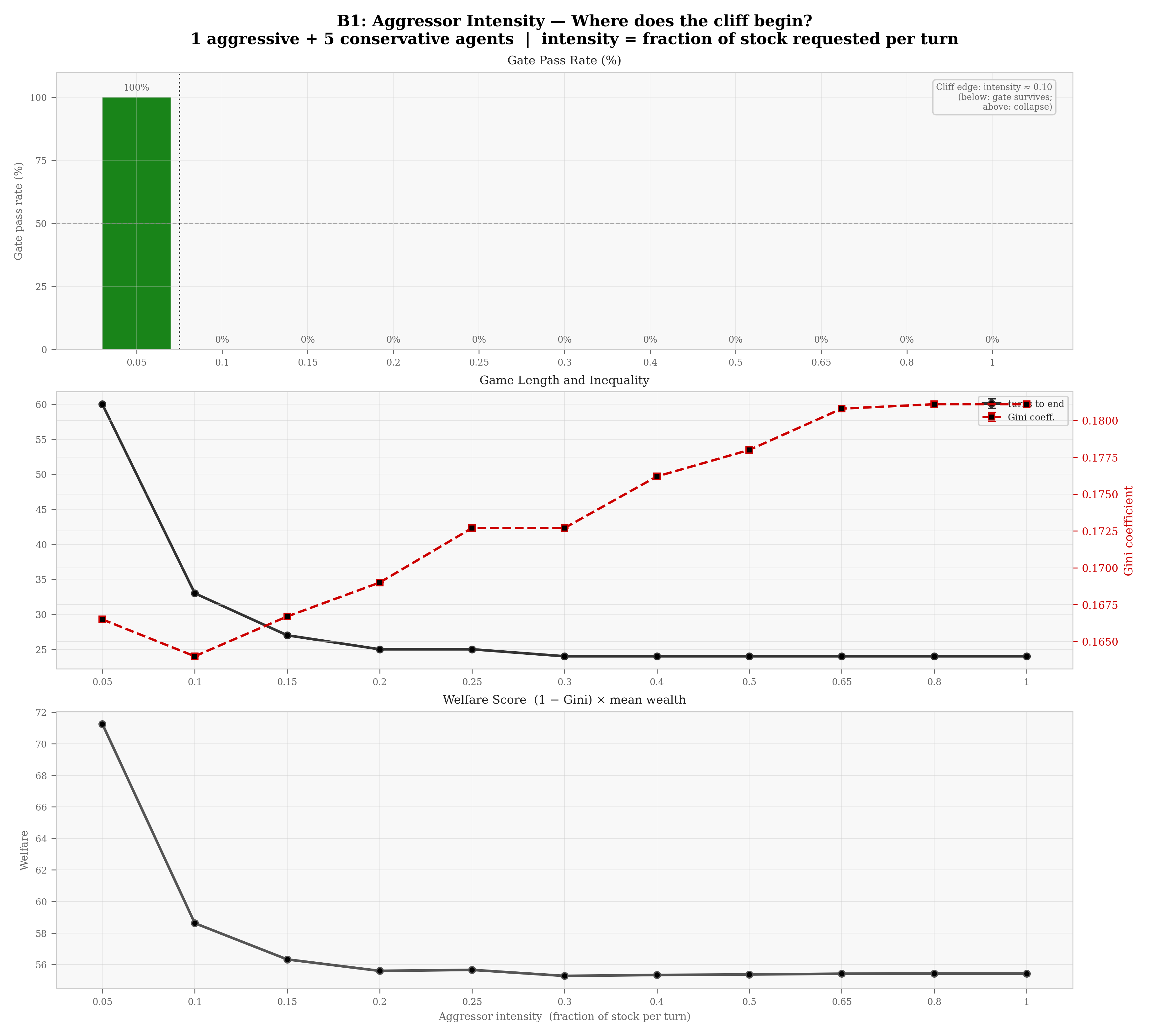
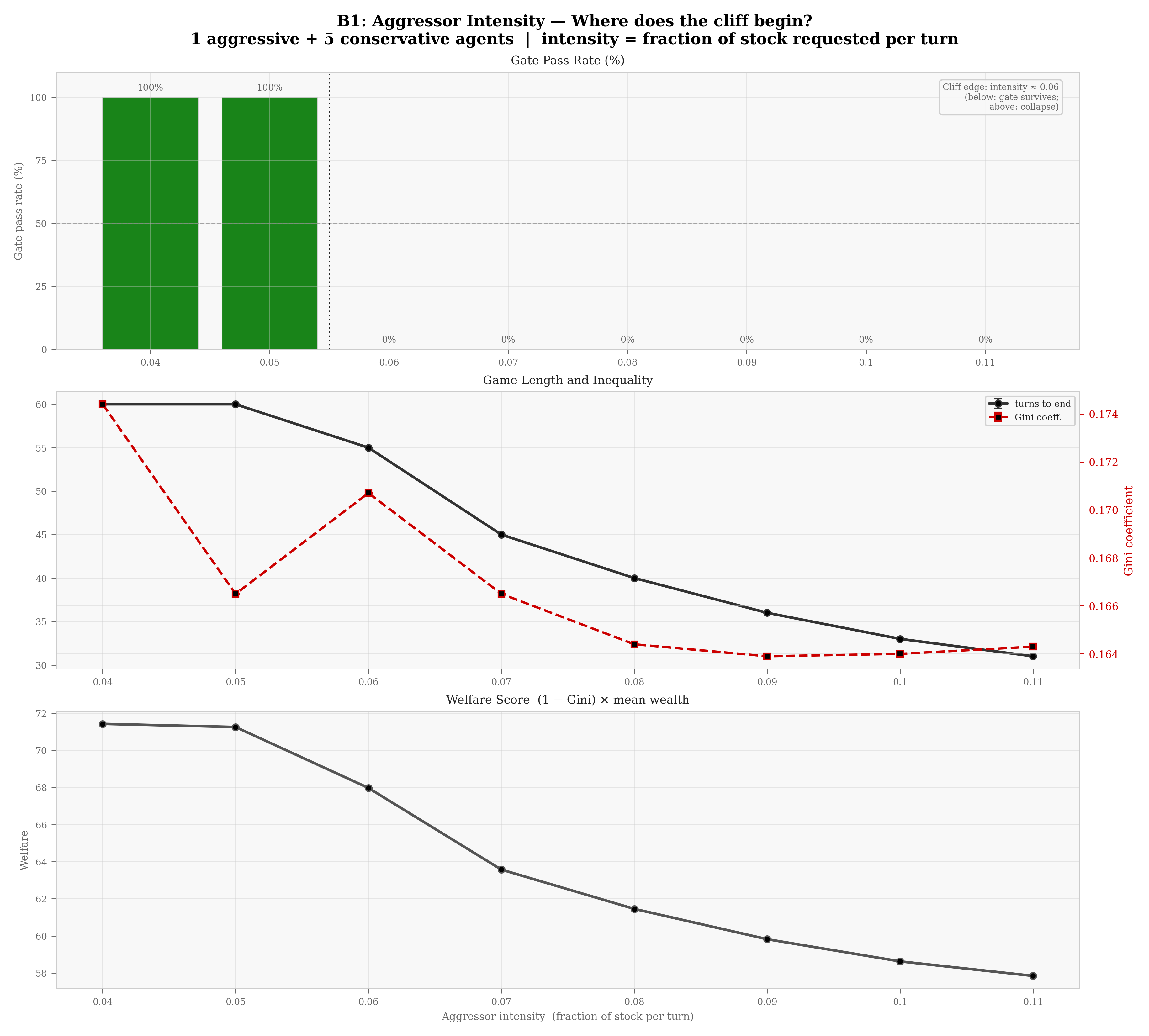
Motivation. The canonical P1 sweep uses the default aggressive heuristic with \(i = 0.5\) (fraction of stock requested per turn). The analysis raised the question of whether the “discontinuous step” might reflect an extreme parametrisation rather than a structural property. B1 sweeps \(i\) from 0.05 to 1.0 (coarse) and from 0.04 to 0.11 (fine, at step 0.01) to identify the precise intensity threshold below which a single aggressor no longer dooms the commons. Population: 1 aggressive + 5 conservative agents, \(r = 0.12\), \(K = 150\), 5–30 runs per cell.
Result. The cliff edge lies at \(i \approx 0.05\)–\(0.06\): at \(i = 0.05\) the gate passes 100%; at \(i = 0.06\) it falls to 0%. The canonical heuristic (\(i = 0.5\)) sits nearly an order of magnitude above this threshold. The step-collapse is therefore not an artefact of an extreme parametrisation — even a minimally extractive aggressor (6% of stock per turn) dooms the commons within the canonical regime. Bootstrap CI on the cliff edge: [0.04, 0.05] (10000 iterations; quantised by the 0.01 fine-grid spacing). The coarse and fine sweeps are shown side-by-side in Figure C.1 (panels Figure C.1 (a) and Figure C.1 (b)).
C.2 B2 — Reactive Reduction Factor: Generalising the Effect
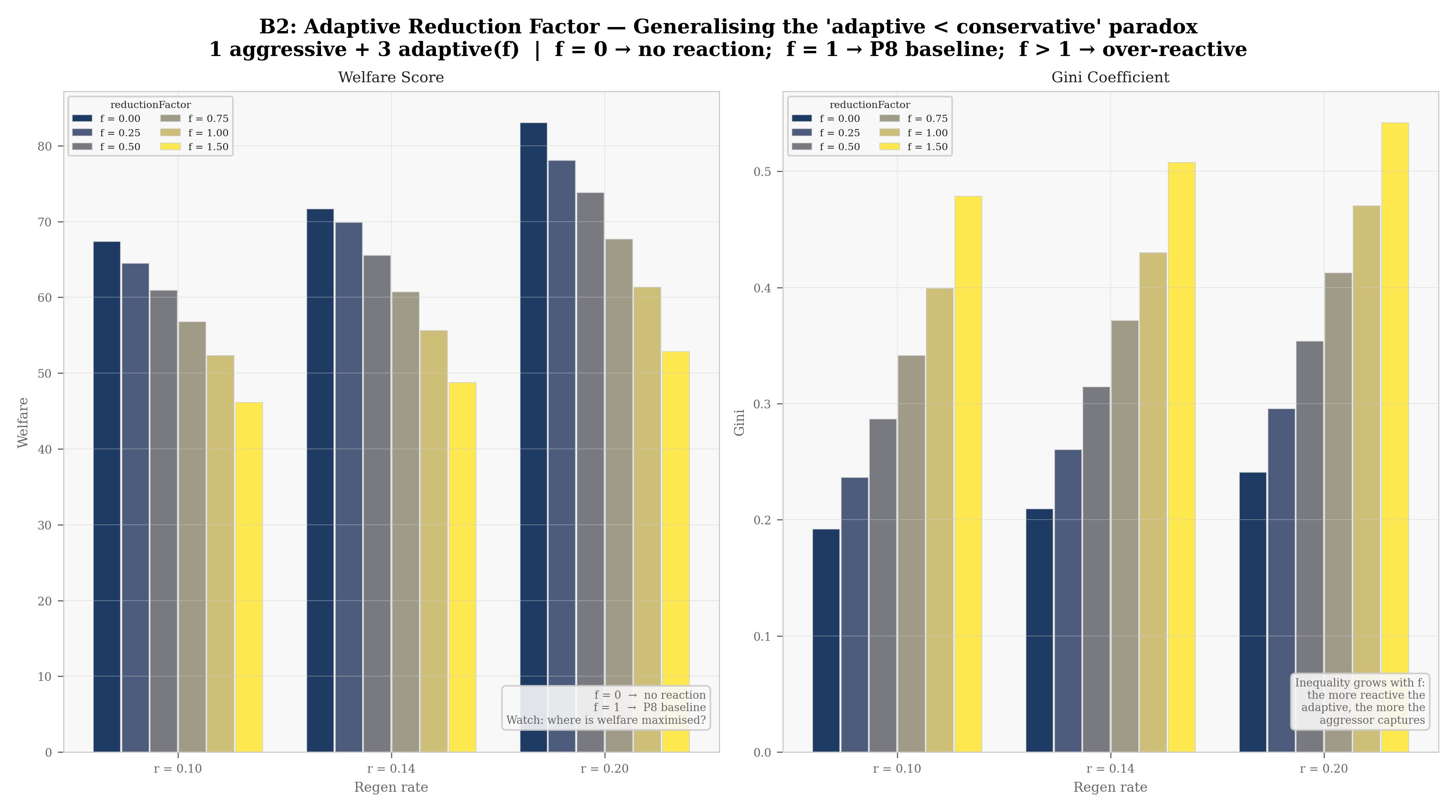
Motivation. The canonical P8 result shows that reactive agents underperform conservative ones. A further question arising from P8 was whether this holds across different strengths of the reactive response, or only for the specific heuristic hardcoded in the platform. B2 introduces a continuous parameter \(f \in [0, 1.5]\) — the reductionFactor — that scales how strongly the reactive agent cuts harvest in response to a falling stock signal (\(f = 0\): no reaction; \(f = 1\): canonical P8 heuristic; \(f > 1\): over-reactive). Population: 1 aggressive (default intensity) + 3 reactive agents, swept at three regen rates (\(r \in
\{0.10, 0.14, 0.20\}\)), 20 runs per cell.
Result. Welfare declines monotonically with \(f\) at all tested regen rates; Gini rises monotonically (Figure C.2). The paradox is not a threshold phenomenon but a graded strategic externality: every unit of reactive response incurs a proportional welfare cost. The slope steepens with \(r\) (higher regen provides more harvest space to concede). All 95% bootstrap CIs on the slope exclude zero.
| Regen rate | Welfare slope per unit \(f\) | 95% bootstrap CI |
|---|---|---|
| \(r = 0.10\) | -14.62 | [-16.39, -13.79] |
| \(r = 0.14\) | -16.17 | [-19.16, -14.26] |
| \(r = 0.20\) | -20.61 | [-22.91, -19.67] |
C.3 B3 — Extended Regen Rate: Identifying the Rescue Boundary
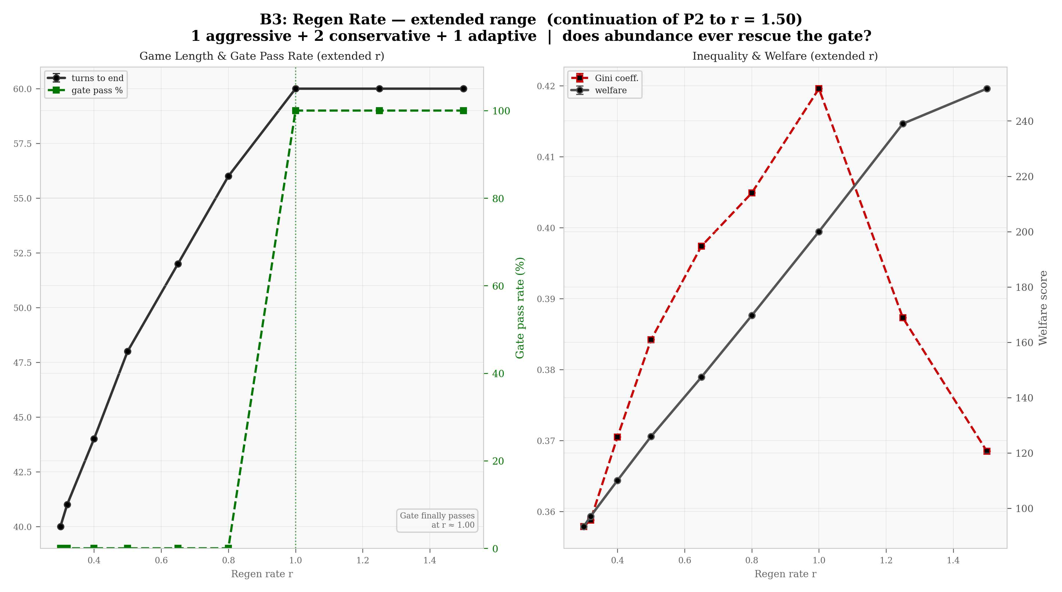
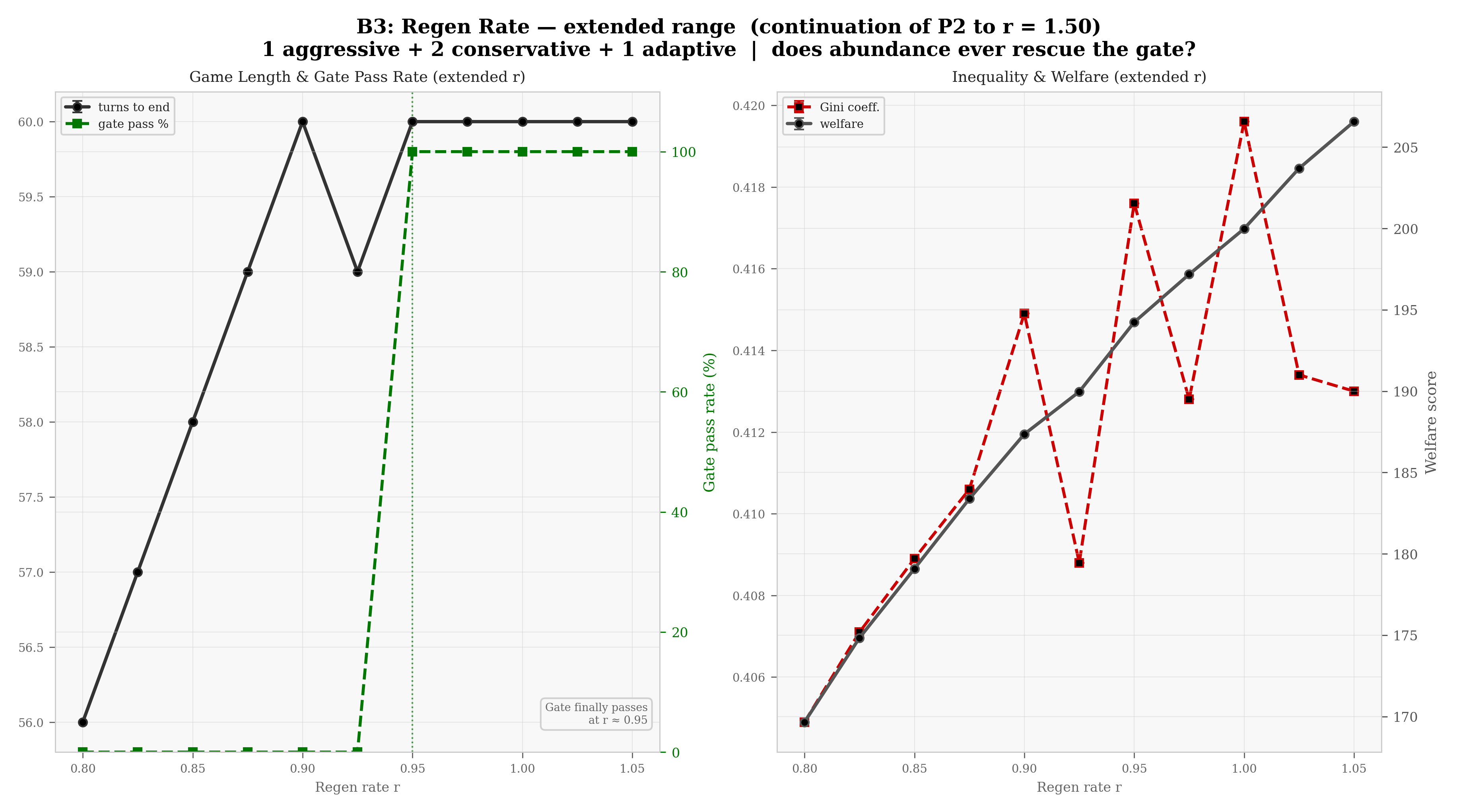
Motivation. P2 sweeps \(r \in [0.04, 0.32]\) and finds gate = 0% throughout, leading to the claim “no level of regeneration offsets a single aggressor.” B3 extends this sweep to \(r = 1.50\) (coarse, irregular grid) and \(r \in [0.80, 1.05]\) (fine, step 0.025) to determine whether a rescue point exists and, if so, precisely where. Population: same as P2 (1 aggressive + 2 conservative + 1 reactive), \(K = 150\), 5–20 runs per cell.
Result. A rescue point exists: gate passage first occurs at \(r \approx 0.95\) (coarse scan: between \(r = 0.80\) (0%) and \(r = 1.00\) (100%); fine scan: transition between \(r = 0.925\) (0%) and \(r = 0.950\) (100%)). Bootstrap CI on rescue point: [0.95, 1.025] (10000 iterations). This boundary lies \(\approx 3\times\) above the canonical CPR maximum (\(r \leq 0.32\); \(0.95/0.32 \approx 3\)) and \(\approx 8\times\) above the default platform regen rate (\(r = 0.12\)), confirming that the original P2 claim is valid within any empirically realistic regime. The coarse and fine sweeps are shown side-by-side in Figure C.3 (panels Figure C.3 (a) and Figure C.3 (b)).
C.4 B4 — Shock Response without an Aggressor: Isolating Resource Dynamics
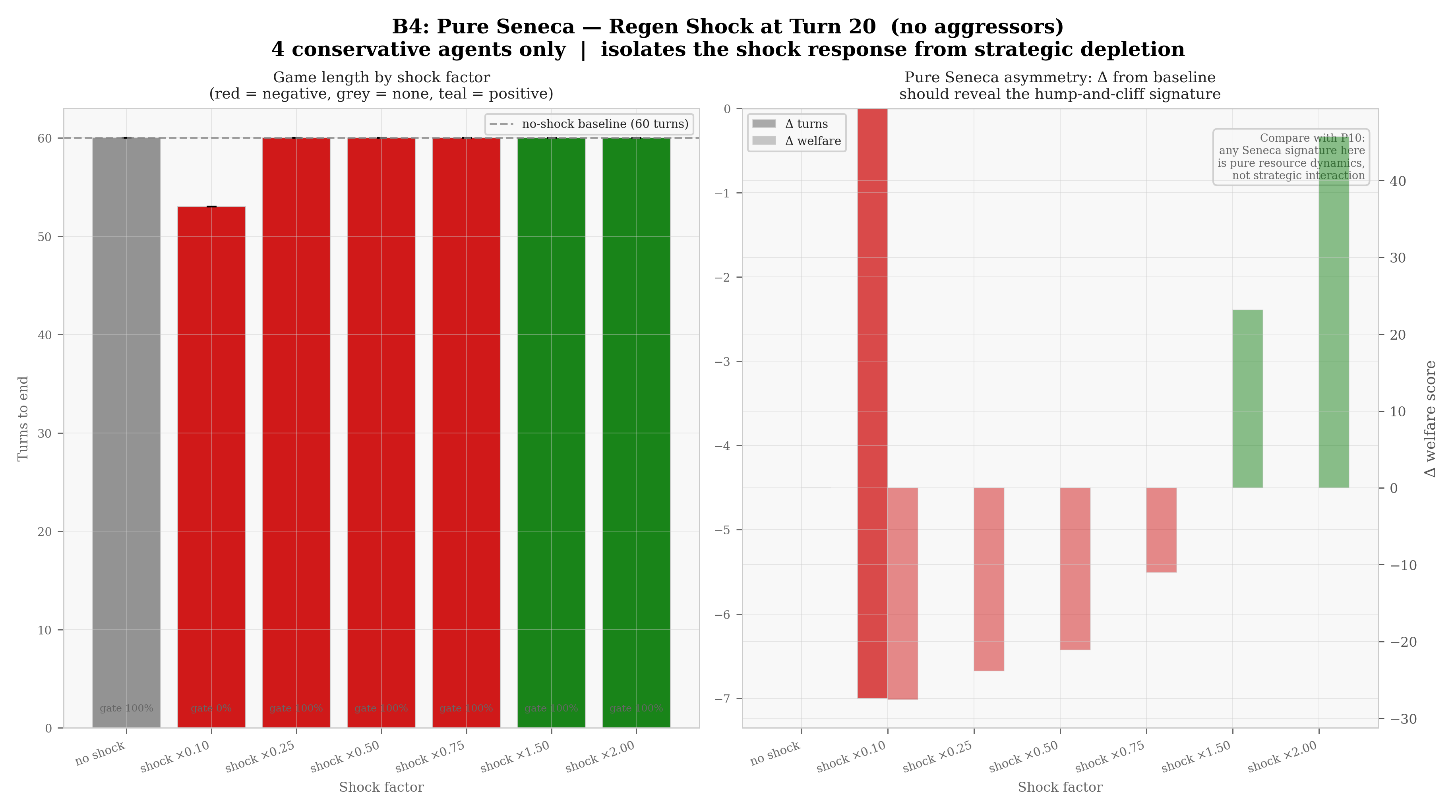
Motivation. P10 finds that negative regen shocks produce only modest, bounded damage while positive shocks provide larger gains — the reverse of the classical Seneca prediction. This inverted pattern could reflect either (a) an intrinsic property of the logistic commons, or (b) the aggressive agent having already pre-committed the system to its depletion trajectory before the shock arrives, so that negative shocks are marginal and positive shocks merely extend a doomed trajectory. B4 removes the aggressive agent entirely — 4 conservative agents, same shock protocol — to isolate component (a). Population: 4 conservative agents, \(r = 0.12\), shock at turn 20, \(f \in \{0.10, 0.25, 0.50, 0.75, 1.00, 1.50, 2.00\}\), 20 runs per cell.
Result. Without strategic pre-depletion, the logistic commons responds proportionally to shocks: negative shocks require severe magnitude (\(f < 0.25\)) to trigger collapse at all (welfare loss \(\approx\) 27.8 points at \(f = 0.10\) due to collapse), and moderate negative shocks (\(f = 0.50\), \(f = 0.75\)) produce moderate, real welfare losses (-21 and -11 points from a baseline of 112.8). Positive shocks provide comparable or larger gains (+23 at \(f = 1.50\), +46 at \(f = 2.00\)). The asymmetry indices confirm that the logistic model has no intrinsic Seneca-direction asymmetry (negative hurting more than positive helps) at any tested magnitude: indices are near zero at moderate magnitudes and positive at extremes — meaning positive shocks provide somewhat more relief than matched negative shocks cause damage, not the reverse.
| Paired shocks | Asymmetry index | Interpretation |
|---|---|---|
| \(f = 0.50\) vs \(f = 1.50\) | +2.0 | Near-symmetric; slight anti-Seneca lean |
| \(f = 0.25\) vs \(f = 1.50\) | -0.7 | Near-symmetric (negligible magnitude) |
| \(f = 0.10\) vs \(f = 2.00\) | +18.2 | Positive shocks help substantially more at extremes |
This contrasts sharply with P10 (aggressive agent present), where the same moderate negative shock (e.g. \(f = 0.50\)) acts on a system already committed to collapse, making its marginal damage negligible. The contrast between the two experiments is therefore not about the resource model — it is about the strategic state of the system at the moment the shock arrives. The full shock-factor response and the near-symmetric \(\Delta\)-panel are shown in Figure C.4.
C.5 B5 — Statistical Inference: Cross-Sweep Analysis
Motivation. The analysis of the first set of experimental results suggested the need for formal statistical backing to support the reported differences. B5 applies retrospective inference to all 17 loaded sweep results (167 cells in total): logistic regression of gate pass rate on canonical covariates, bootstrap CIs for threshold locations, and permutation tests for stochastic sweeps.
Variance audit. All platform sweeps except two are deterministic (zero intra-cell variance), reflecting the deterministic nature of the built-in heuristics under a fixed scheduler. Only observability_noise (max \(\sigma = 0.85\)) and scheduler_comparison (max \(\sigma = 0.66\)) exhibit stochastic variance. For deterministic sweeps, inference is performed at the between-cell level via bootstrap (resampling cells). This audit applies to platform sweeps only; card-tournament sweeps (CT1–CT5) are inherently stochastic (Forest Die rolls, deck shuffles, mandatory-defection draws) and are sampled at \(n = 200\) games per cell to control this variance — see §3.3.
aggressive_fraction would likely absorb this effect.
| Predictor | Coefficient | 95% Bootstrap CI | Robust? |
|---|---|---|---|
| aggressor intensity | -67.4 | [-130.4, +0.8] | Borderline |
| regen rate | +40.3 | [+23.8, +77.3] | \(\checkmark\) |
| aggressive count | -32.9 | [-63.6, -19.7] | \(\checkmark\) |
| reactive reductionFactor | -6.4 | [-36.3, +2.9] | \(\times\) |
| pool size (\(n\) agents) | +1.8 | [+0.9, +4.0] | \(\checkmark\) |
C.5.1 Cross-Sweep Logistic Regression
A binomial GLM was fitted to the 167-cell pooled dataset (outcome: gate successes out of \(n\) replicates; predictors: aggressor intensity, regen rate, aggressive count, reactive reductionFactor, pool size). Bootstrap CIs (10000 iterations resampling cells) are reported alongside model estimates; for deterministic sweeps, the bootstrap CI is more reliable than the model standard error. The same coefficients with their bootstrap intervals are visualised in Figure C.5.
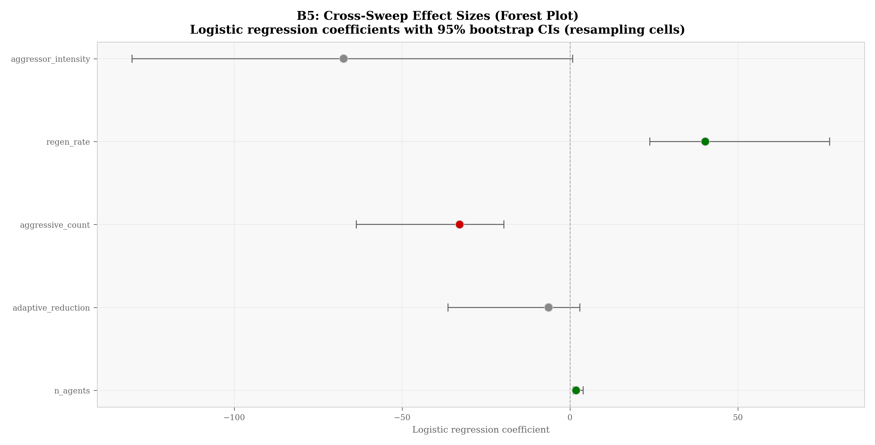
aggressor_intensity is borderline (CI upper bound = +0.8, direction correct). The two green predictors reflect structural features of the system: more regeneration and larger dilution of the single aggressive agent both shift the equilibrium towards gate survival.
C.5.2 Sweep-Specific Bootstrap CIs
| Experiment | Observed threshold | 95% Bootstrap CI | Source sweep |
|---|---|---|---|
| B1 cliff edge (last \(i\) with gate > 50%) | 0.050 | [0.040, 0.050] | aggressive_intensity_sweep_fine |
| B3 rescue point (first \(r\) with gate > 50%) | 0.950 | [0.950, 1.025] | regen_rate_extended_fine |
B2 welfare slopes (10000 iterations, resampling cells within each regen stratum):
| Regen rate | Slope (welfare per unit \(f\)) | 95% CI |
|---|---|---|
| \(r = 0.10\) | -14.62 | [-16.39, -13.79] |
| \(r = 0.14\) | -16.17 | [-19.16, -14.26] |
| \(r = 0.20\) | -20.61 | [-22.91, -19.67] |
All slopes exclude zero, confirming the monotonic strategic externality of the reactive response across all tested regen rates.
C.5.3 P7 Scheduler Permutation Test
| Metric | Scheduler means | Observed statistic | \(p\)-value | Conclusion |
|---|---|---|---|---|
| Gate pass rate | all 0% | 0.000 | 1.000 | Not distinguishable |
| Game length (turns) | 27.0 / 27.5 / 27.8 | 0.332 | 1.000 | Not distinguishable |
| Welfare score | 69.1 / 68.2 / 68.1 | 0.544 | 1.000 | Not distinguishable |